

DMTN-171
Fall 2020 status of crowded field processing with the LSST Alert Production Pipelines#
Abstract
A report on the Fall 2020 state of the LSST Alert Production Pipelines’ ability to process deep images in the galactic bulge.
Introduction#
Some of the earliest applications of image differencing in astronomy were motivated by the desire to identify transient sources (microlensing events) in extremely crowded stellar fields. At ground-based photometric precision, typically about one percent of stellar sources have detectable variability. Thus by subtracting a coadded historical (template) image from a new (science) image, the crowding can be reduced by a factor of ~100.
In this technote we assess the state of crowded field processing in Fall 2020 using the LSST Alert Production (AP) Science Pipelines [Rubin Observatory Science Pipelines Developers, 2025]. Alert Production uses image differencing to identify transient, moving, and variable sources in LSST images within 60 seconds of camera readout. Crucially, the AP processing must meet its requirements even in the most crowded fields it will encounter. Of particular importance are the transient reporting latency (OTT1 and OTR1; LSR-REQ-0117 and LSR-REQ-0025), the reliability with which images are processed (sciVisitAlertDelay and sciVisitAlertFailure; OSS-REQ-0112), the photometric and astrometric accuracy of the resulting catalogs (dmL1AstroErr, dmL1PhotoErr, and photoZeroPointOffset; OSS-REQ-0149 and OSS-REQ-0152), completeness and purity metrics for transients (OSS-REQ-0353) and solar system objects (OSS-REQ-0354), and source misassociation for transients (OSS-REQ-0160) and solar system objects (OSS-REQ-0159). The full requirement text can be found in Claver and The LSST Systems Engineering Integrated Project Team [2017] and Claver and The LSST Systems Engineering Integrated Project Team [2018]. Accordingly, large-scale tests on precursor datasets are necessary to identify where improvements are needed in order to meet requirements. The status of the processing also will inform ongoing cadence planning for the overall survey.
The scope of this technote does not include obtaining photometry for static sources in direct images (except insofar as it is required to conduct image differencing), nor comparisons to dedicated crowded field processing codes. DMTN-077 addresses those issues.
Overview of the data#
To test the LSST Science Pipelines on crowded fields, we acquired public data from the DECam survey of the galactic bulge by Saha et al. [2019].
The full survey consists of six fields at low galactic latitudes observed in the six ugrizy bands, though for this investigation we limited the analysis to g- and i-bands for the two fields closest to the galactic center (B1 and B2, Table 1).
The two fields selected for this test were observed in 2013 and 2015 to similar depth in both bands (Table 2).
These data are available on lsst-devl at /datasets/decam, while the processed data is available in /project/sullivan/saha2.
The size of the processed data amounts to 7.0Tb on disk, which can be fully recreated using release 21.0 of the Science Pipelines following the instructions in that directory, which have also been copied to https://github.com/lsst-dm/dmtn-171/processing_scripts for public access.
Field |
RA |
Dec |
Galactic longitude |
Galactic latitude |
|---|---|---|---|---|
B1 |
\(270.8917^{\circ}\) |
\(-30.0339^{\circ}\) |
\(1.02^{\circ}\) |
\(-3.92^{\circ}\) |
B2 |
\(272.3500^{\circ}\) |
\(-31.4350^{\circ}\) |
\(0.40^{\circ}\) |
\(-5.70^{\circ}\) |
Field |
band |
2013 |
2015 |
|---|---|---|---|
B1 |
g |
30 |
44 |
B2 |
g |
31 |
44 |
B1 |
i |
53 |
44 |
B2 |
i |
49 |
44 |
It is important to note that the seeing was uniformly worse in 2013 than in 2015 for this survey (Fig. 1 - Fig. 4).
As a result, we expect image differencing to fare much worse when running ap_pipe on the 2015 observations using the template constructed from the 2013 observations.
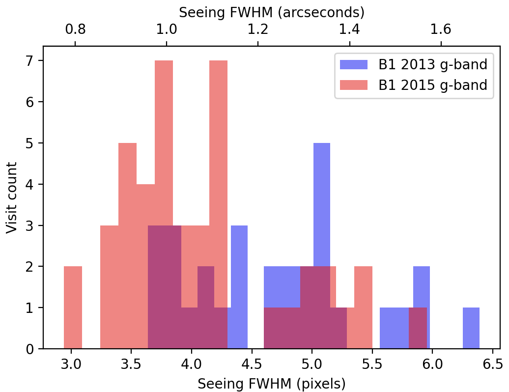
Fig. 1 Distribution of seeing for g-band observations of field B1#
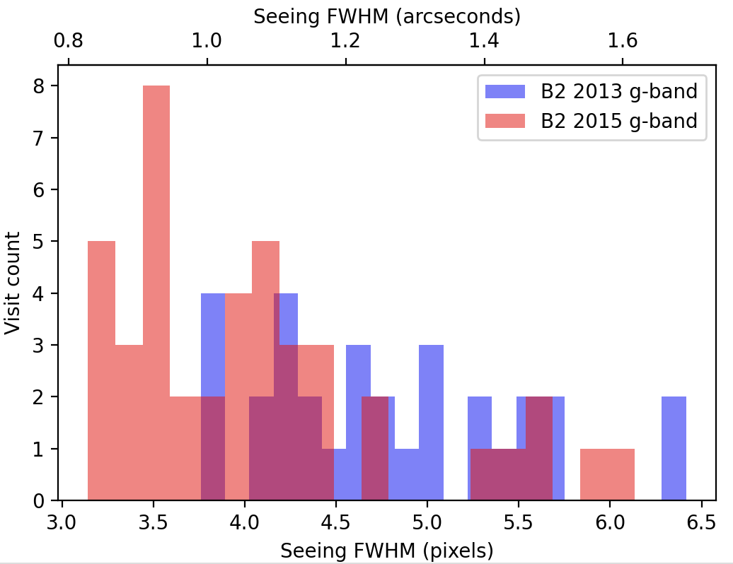
Fig. 2 Distribution of seeing for g-band observations of field B2#
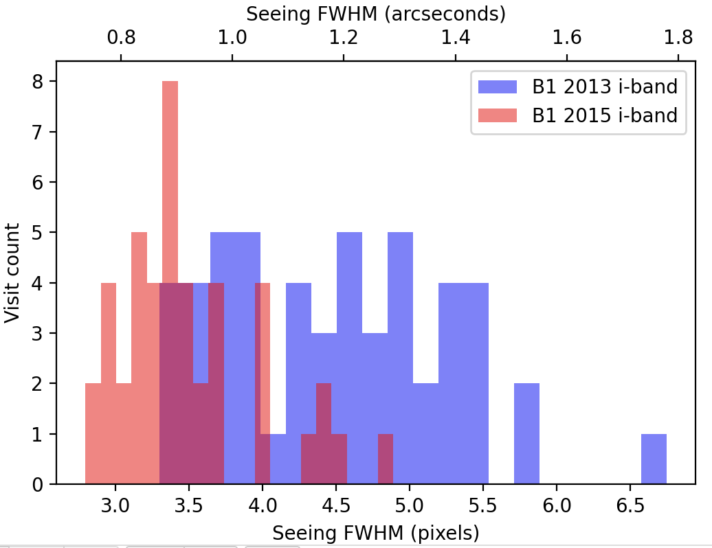
Fig. 3 Distribution of seeing for i-band observations of field B1#
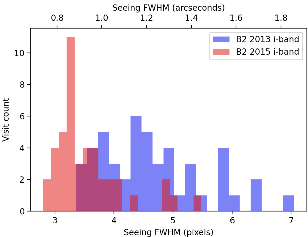
Fig. 4 Distribution of seeing for i-band observations of field B2#
Running the Science Pipelines#
Running the LSST Science Pipelines on observations of crowded fields follows the same steps as for fields with lower densities, but in this investigation a few of those steps required modification to work properly. Here, we divide processing into three distinct stages:
Single Frame Processing: includes applying flat field and bias corrections, Instrument Signature Removal, and astrometric and photometric calibration.
Coaddition: includes warping and PSF-matching the individual exposures, as well as the actual coaddition algorithm.
Alert Production: includes all of Single Frame Processing for the science images, as well as warping the templates, performing image differencing, detecting and measuring sources, and associating sources from different visits to form objects.
Single Frame Processing#
The initial stages of Single Frame Processing required no modifications to accommodate crowded fields. In source detection, however, it became necessary to set the detection threshold to a fixed value rather than the default of a multiple of the standard deviation of the background. There may be no pixels without a detectable source in the exposures, so the measured background level will be incorrect and the number of sources used for PSF modeling will be unpredictable, and possibly too few. For this test, we took typical detection thresholds from DECam HiTS observations and found that those eliminated the related processing errors. Further refinement would likely yield improved results. All of the modifications needed to run single frame processing on these data can be found in Table 3, below.
Modified config settings for processCcd.py |
value |
band |
|---|---|---|
charImage.requireCrForPsf |
False |
i, g |
charImage.detection.thresholdValue |
10000 |
i |
charImage.detection.thresholdValue |
2500 |
g |
charImage.detection.includeThresholdMultiplier |
1.0 |
i, g |
charImage.detection.thresholdType |
“value” |
i, g |
charImage.repair.cosmicray.nCrPixelMax |
10000000 |
i, g |
charImage.repair.cosmicray.min_DN |
10000 |
i |
charImage.repair.cosmicray.min_DN |
2500 |
g |
Beyond the source detection thresholds, it was necessary to modify two additional components. We found that the default algorithm for measuring the PSF, a simple PCA-based model, simply failed when run on most of the visits from these crowded fields. However, PSFex was able to successfully measure the PSF, and since it was already supposed to be the default in the Science Pipelines (per RFC-312) we carried out that overdue implementation for all cameras. Thus, no further modifications are needed for future processing.
The final component that required modification is the cosmic ray detection and repair algorithm.
As noted above, the assumptions behind the pixel value statistics are incorrect in crowded fields.
We set the detection thresholds to the same values as for source detection (Table 3), and while this works in most cases, for just under 1% of the exposures processCcd.py fails with a fatal error.
In these cases the failure appears to be due to every pixel in the image being identified as a cosmic ray.
This failure suggests that our cosmic ray detection algorithm needs improvement and should be investigated further, but because of the low number of exposures affected we simply increased the number of pixels required to trigger the failure.
This does not solve the problem, but it allows us to continue processing these exposures to make sure that there are no additional problems.
Evaluation of the Point Spread Function (PSF)#
The accuracy of the measurement of the Point Spread Function (PSF) is our greatest concern with processing crowded fields, since it is typically not possible to find a sufficient number of isolated stellar sources to measure. The PSF is used for very little in the current Science Pipelines; our standard Alard&Lupton-style image differencing depends only on the calculated size of the PSF to compare with that of the template, and not on the shape of the PSF. However, the accuracy of the PSF does impact source measurement.
In Fig. 5 through Fig. 12 below, we show the PSF for every visit for CCD 42, located near the center of the focal plane. The color scale is set to highlight features in the wings with a square root stretch, while contours at logarithmic intervals capture the shape of the core of the PSF. Each PSF is normalized to have a sum of 1, and the same color scale and contour levels are used for every image.
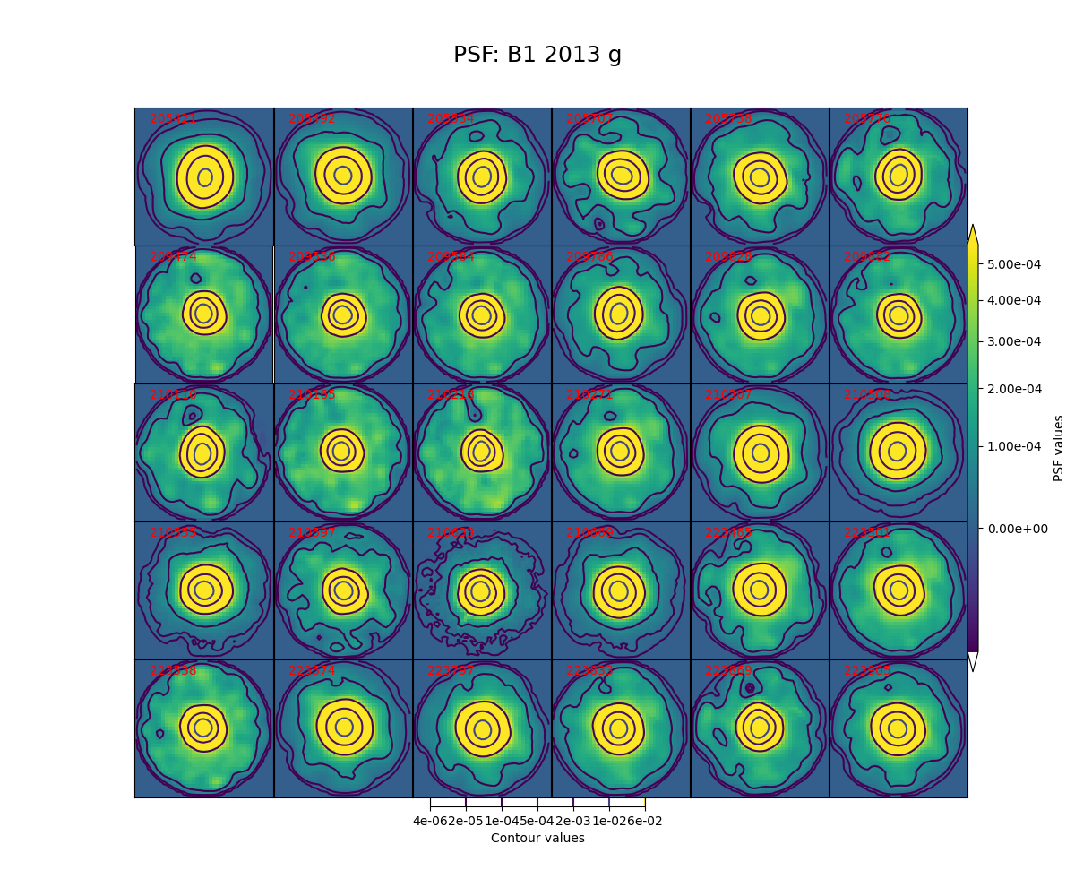
Fig. 5 PSFs for each of the g-band visits from 2013 in field B1, for a CCD in the center of the focal plane.#
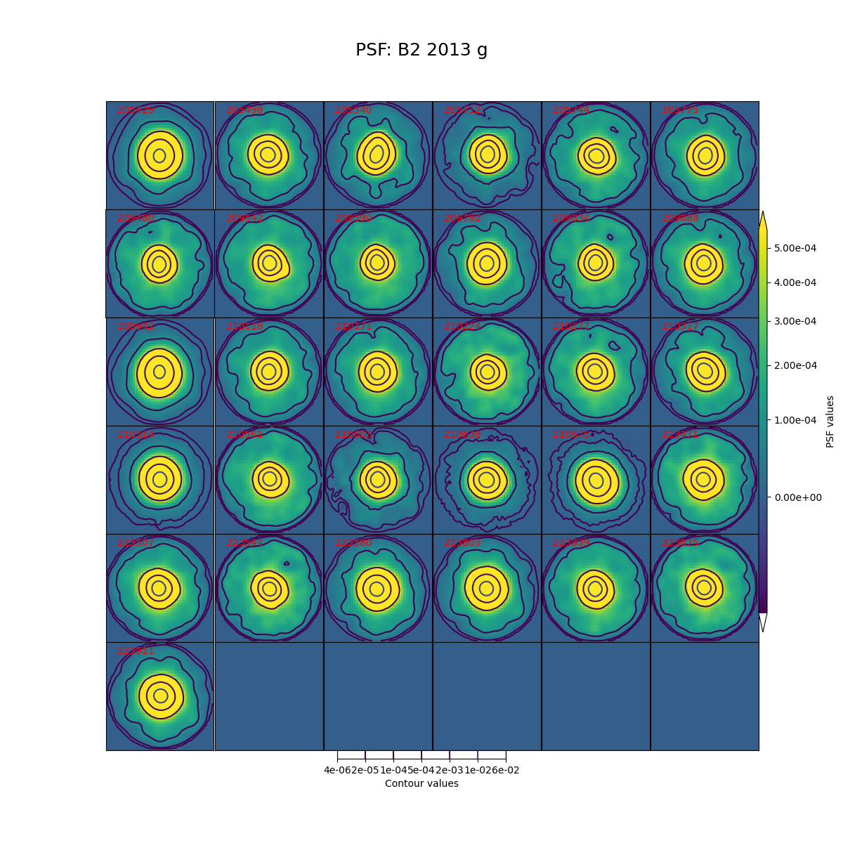
Fig. 6 PSFs for each of the g-band visits from 2013 in field B2, for a CCD in the center of the focal plane.#
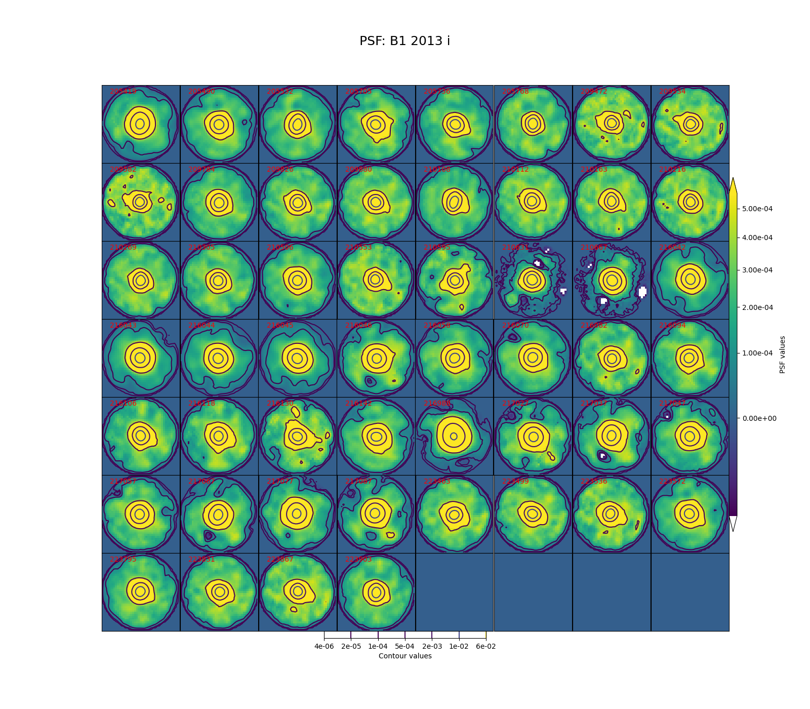
Fig. 7 PSFs for each of the i-band visits from 2013 in field B1, for a CCD in the center of the focal plane.#
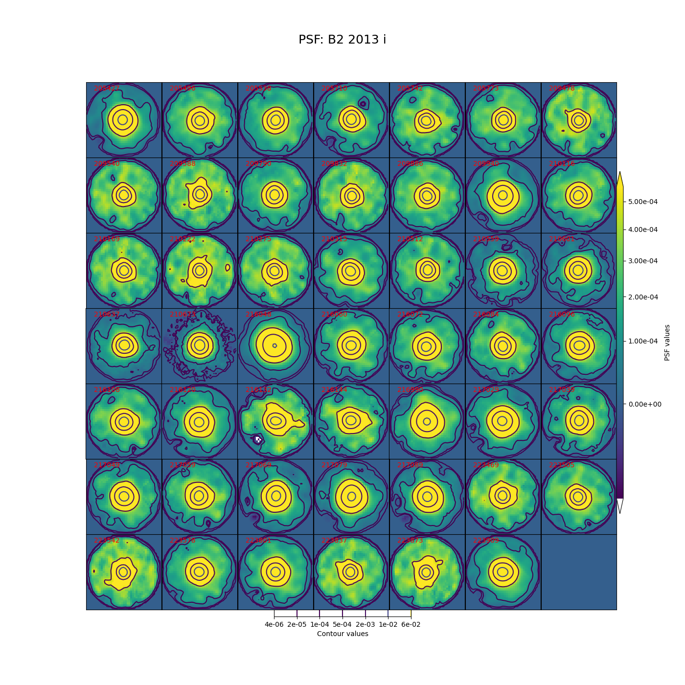
Fig. 8 PSFs for each of the i-band visits from 2013 in field B2, for a CCD in the center of the focal plane.#
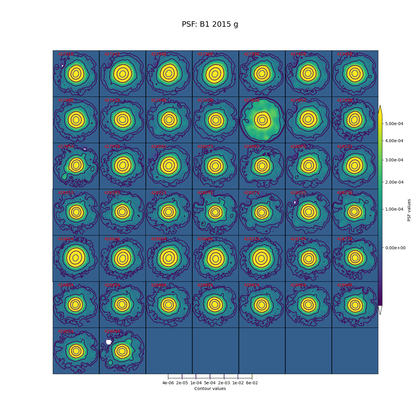
Fig. 9 PSFs for each of the g-band visits from 2015 in field B1, for a CCD in the center of the focal plane.#
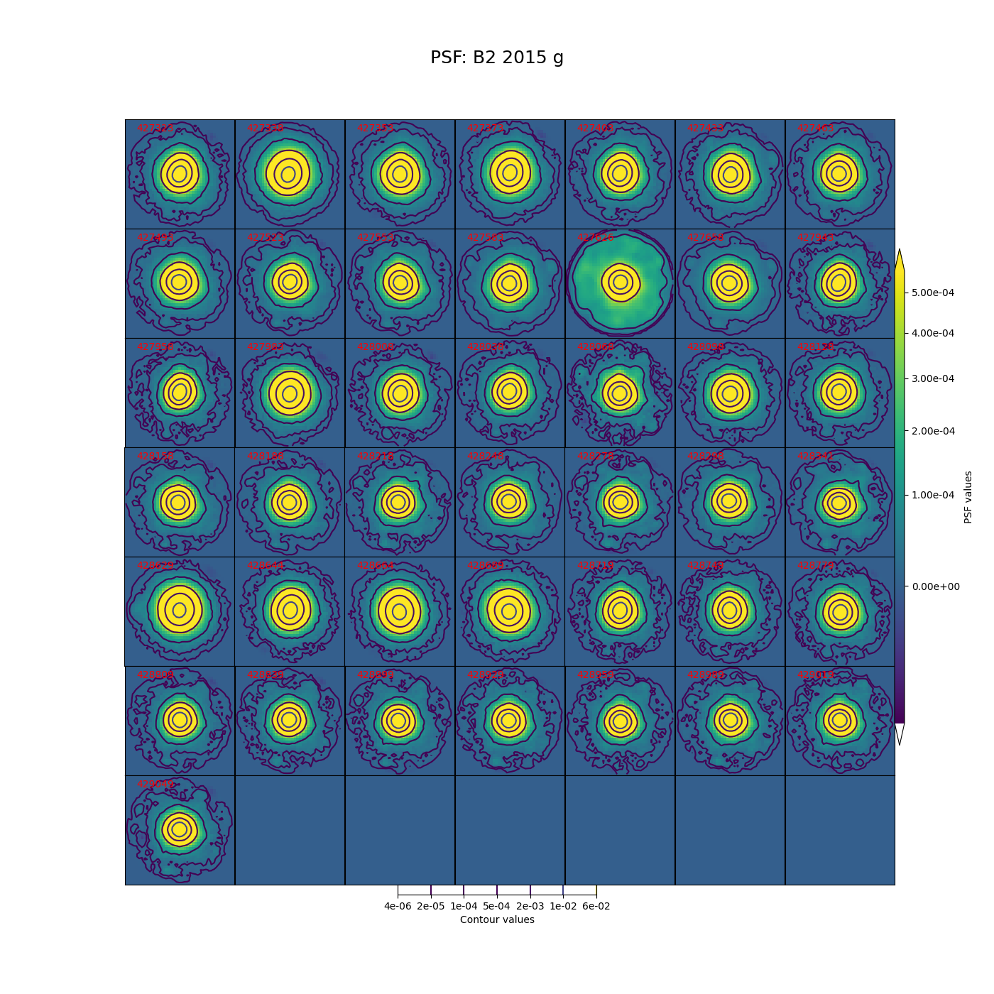
Fig. 10 PSFs for each of the g-band visits from 2015 in field B2, for a CCD in the center of the focal plane.#
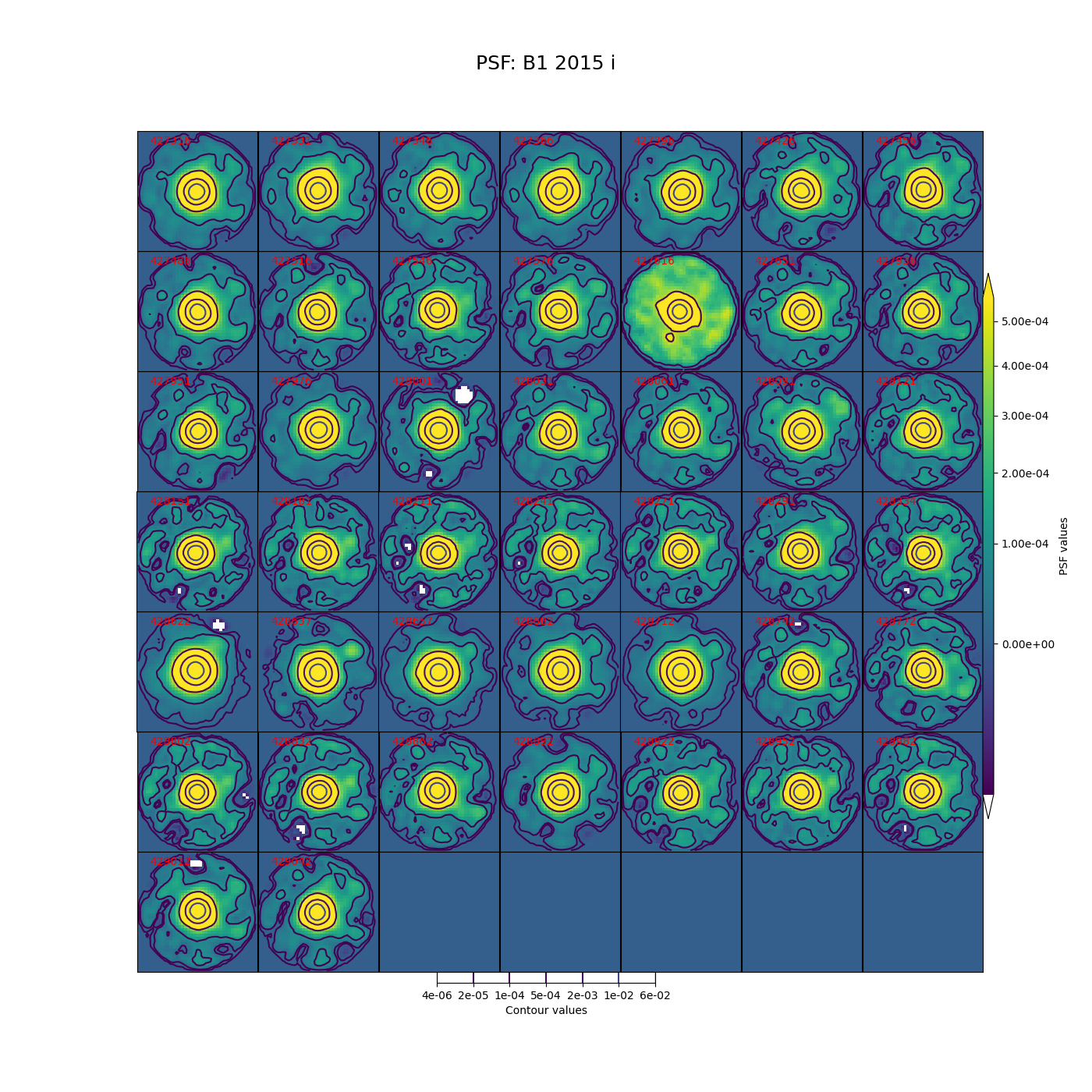
Fig. 11 PSFs for each of the i-band visits from 2015 in field B1, for a CCD in the center of the focal plane.#
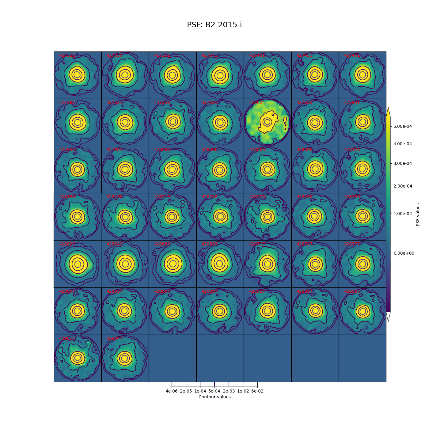
Fig. 12 PSFs for each of the i-band visits from 2015 in field B2, for a CCD in the center of the focal plane.#
While g-band generally has clean and reasonably symmetric-looking PSFs, some i-band visits show worrisome features in the wings of the PSF. As noted above, these are not likely to impact the performance of Alert Production, though it is undesirable. For these crowded fields, our current PSF modeling algorithm PSFex is sufficient to run Alert Production, but a more robust algorithm would be desirable.
Density of measured sources on a single ccd#
In DMTN-077 a significant drop was seen in the fraction of sources detected with the 2017 Science Pipelines compared to processing of the same fields in the DECam Plane Survey (DECAPS) [Schlafly et al., 2018]. In that analysis, the very crowded region with 500k sources per square degree in DECAPS had only 200k sources detected per square degree when processed with the Science Pipelines, suggesting that the Science Pipelines processing was missing many faint sources. While we do not have an externally-produced catalog of the same field to compare against, we do measure a significantly higher density of sources than was seen in that analysis, roughly in line with the DECAPS results. In figures Fig. 13 through Fig. 16 below, we plot histograms of the number of sources detected in single frame measurement for a single ccd across all visits. The chosen ccd lies roughly in the center of the focal plane, and has an average density of sources for the field. These histograms exclude any sources flagged as being saturated, too close to an edge of the ccd, or contaminated by a cosmic ray. The wide distribution seen for each field is believed to be due to the range of seeing throughout the observations (Fig. 1 - Fig. 4).
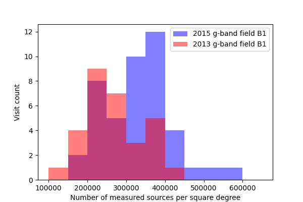
Fig. 13 Density of detected sources across all visits for field B1 in g-band, for ccd 42.#
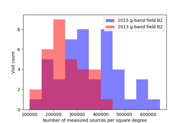
Fig. 14 Density of detected sources across all visits for field B2 in g-band, for ccd 42.#
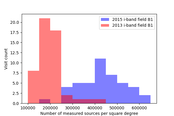
Fig. 15 Density of detected sources across all visits for field B1 in i-band, for ccd 42.#
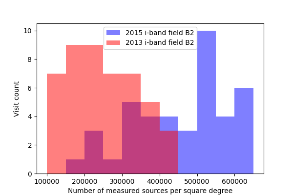
Fig. 16 Density of detected sources across all visits for field B2 in i-band, for ccd 42.#
Source counts#
For a more in-depth look at the performance of the Science Pipelines, we should look at the source counts as a function of magnitude. From these, it should be apparent if the broad range in the density of sources seen in Fig. 13 - Fig. 16 is consistent with varying depth due to seeing, and whether we are systematically undercounting faint sources as suggested by Figure 8 of DMTN-077. In Fig. 17 - Fig. 24 below we plot the source counts as a function of magnitude, separated by year, field and band. Since there are on the order of 40 visits included in each plot, we do not include a legend but instead list the visits with anomalous source counts in Table 4. Those visits appear to have the same features as the others, but are shifted by several magnitudes brighter or fainter, indicating a photometric calibration error. It is noteworthy that all of the anomalous visits in 2015 were taken sequentially, and all but two of the anomalous visits in 2013 were taken sequentially. The two exceptions in 2013 are 216988 and 216048, but these have very poor seeing at 7.56 and 8.11 pixels, respectively, which explains their unusually shallow depth. With the exception of those anomalous visits, the source counts are consistent within each band and field for each observing season, and exhibit the same features at the same magnitudes up to each visits’ cutoff.
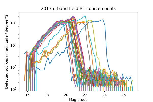
Fig. 17 Source counts for all visits in 2013 for field B1 in g-band, for ccd 42. Visits with an apparant photometric offset are listed in Table 4.#
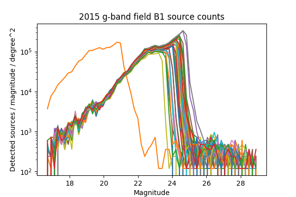
Fig. 18 Source counts for all visits in 2015 for field B1 in g-band, for ccd 42. Visits with an apparant photometric offset are listed in Table 4.#
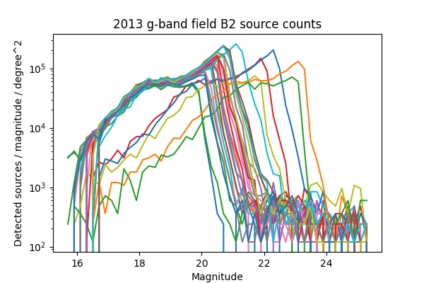
Fig. 19 Source counts for all visits in 2013 for field B2 in g-band, for ccd 42. Visits with an apparant photometric offset are listed in Table 4.#
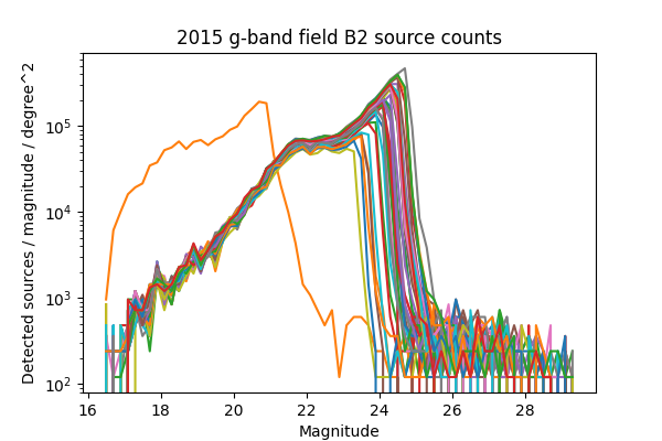
Fig. 20 Source counts for all visits in 2015 for field B2 in g-band, for ccd 42. Visits with an apparant photometric offset are listed in Table 4.#
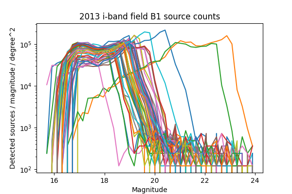
Fig. 21 Source counts for all visits in 2013 for field B1 in i-band, for ccd 42. Visits with an apparant photometric offset are listed in Table 4.#
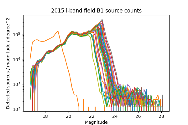
Fig. 22 Source counts for all visits in 2015 for field B1 in i-band, for ccd 42. Visits with an apparant photometric offset are listed in Table 4.#
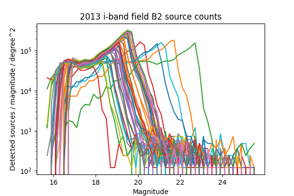
Fig. 23 Source counts for all visits in 2013 for field B2 in i-band, for ccd 42. Visits with an apparant photometric offset are listed in Table 4.#
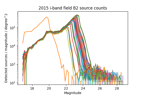
Fig. 24 Source counts for all visits in 2015 for field B2 in i-band, for ccd 42. Visits with an apparant photometric offset are listed in Table 4.#
Year |
Band |
Field |
Visits |
Plot link |
|---|---|---|---|---|
2013 |
g |
B1 |
210508, 210555, 210597, 210633, 210669 |
|
2015 |
g |
B1 |
427628 |
|
2013 |
g |
B2 |
209942, 210514, 210603, 210639, 210675 |
|
2015 |
g |
B2 |
427626 |
|
2013 |
i |
B1 |
210631, 210667, 216988 |
|
2015 |
i |
B1 |
427616 |
|
2013 |
i |
B2 |
210559, 210601, 210637, 210673, 216048 |
|
2015 |
i |
B2 |
427624 |
Timing#
A final concern is the amount of time it will take to process each ccd in crowded fields. While a typical ccd took just under 4 minutes to process, there was a long tail of ccds that took far longer (Fig. 25 and Fig. 26). The increased time was entirely spent in two steps: matching the detected objects to a reference catalog, and measuring the difference image sources. The time required for matching appeared to be non-linear, with the ccds with the largest number of sources and reference objects to match requiring up to four hours to complete. Our matching algorithm was not optimized for these very large numbers of sources, however, so we are encouraged by the results even if the performance is slow.
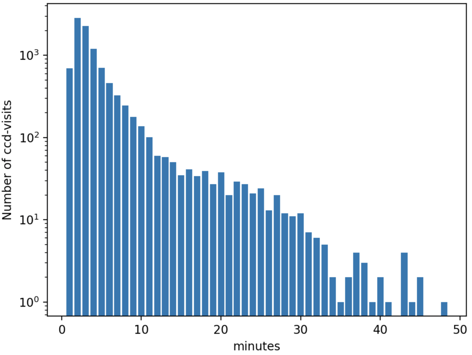
Fig. 25 Distribution of the time required to process each ccd, including both g- and i-band from 2013. Not shown are several ccds that took longer than an hour.#
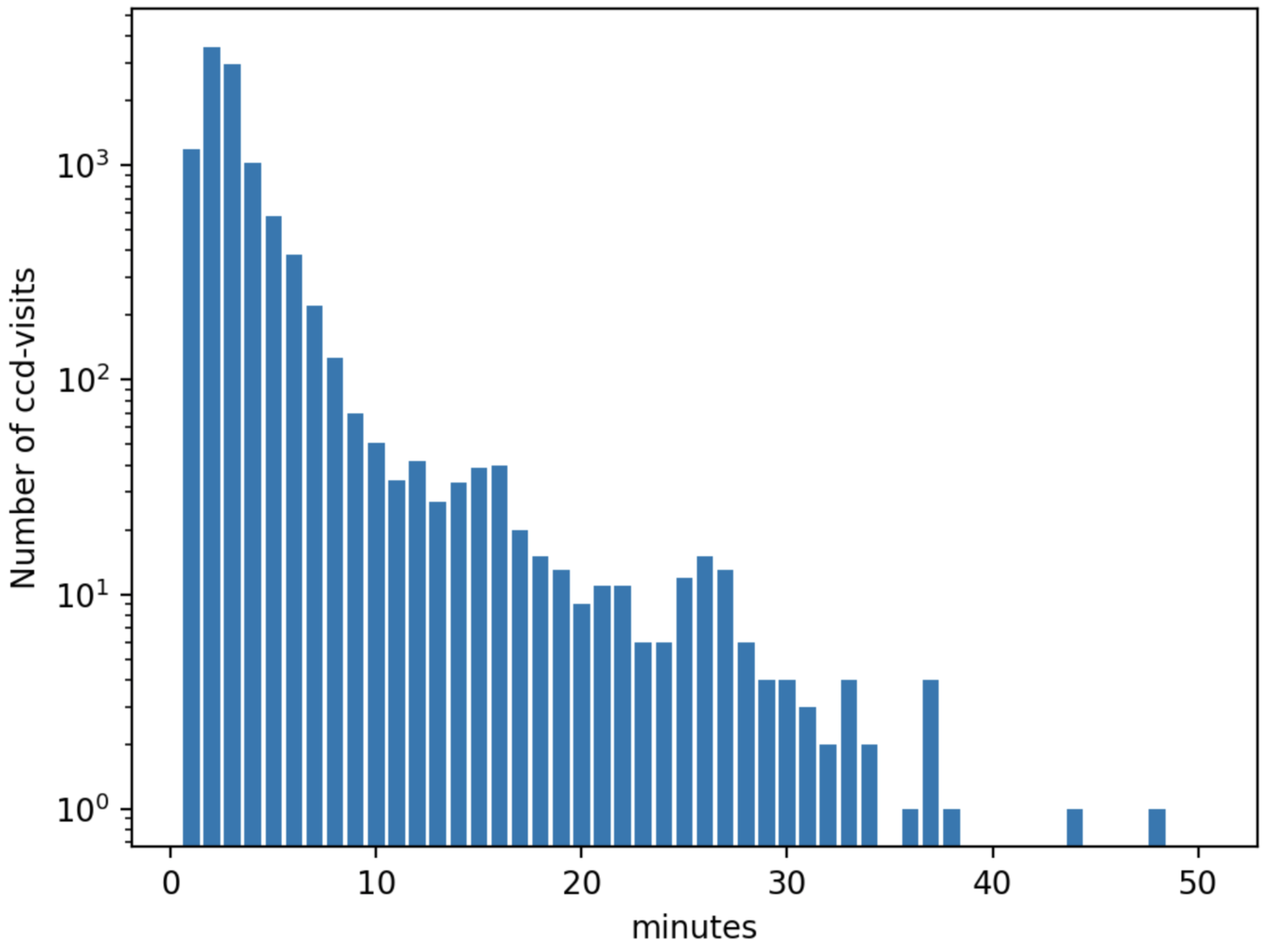
Fig. 26 Distribution of the time required to process each ccd, including both g- and i-band from 2015. Not shown are several ccds that took longer than an hour.#
Warping and coaddition#
While warping and coaddition are significant components of the Science Pipelines, neither is challenged by high stellar density. No modifications were needed to build deep coadded templates for these fields, and no work is anticipated to be needed to support future processing of crowded fields. In Fig. 27 - Fig. 34 below, we show the full mosaic [*] of the two overlapping fields for each band and year separately. We also include the diagnostic N-images, which count the number of visits that contributed to each pixel in the coadd. From these images, we can see that the coverage across the two fields is close to uniform. The small regions where the two fields overlap show a corresponding increase in the nImage count, while the coadded images themselves appear continuous. There are gaps in places in the nImages, but these reflect known chip defects and the saturated cores and wings of bright stars, which are expected. This analysis did not invlove any full-focal plane astrometry or background fitting, so it is noteworthy that the background appears smooth and continuous.
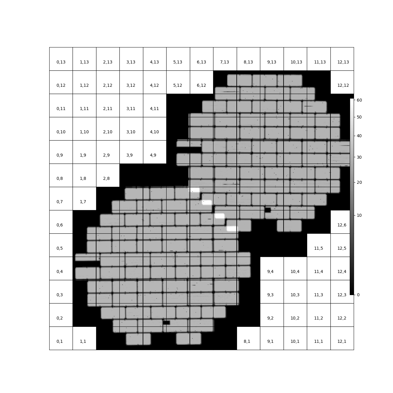
Fig. 27 Overview mosaic of the number of g-band images coadded for both fields from 2013.#

Fig. 28 Overview mosaic of the g-band coadded deep images for both fields from 2013.#
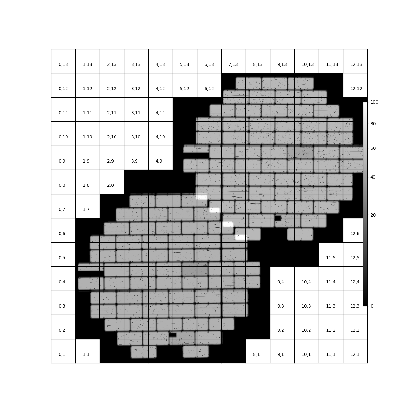
Fig. 29 Overview mosaic of the number of i-band images coadded for both fields from 2013.#
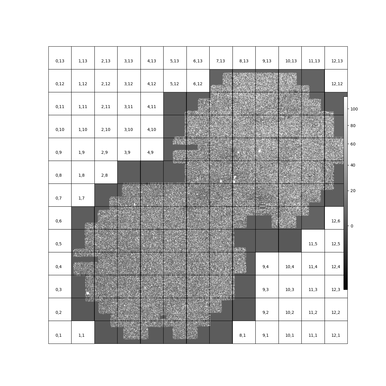
Fig. 30 Overview mosaic of the i-band coadded deep images for both fields from 2013.#
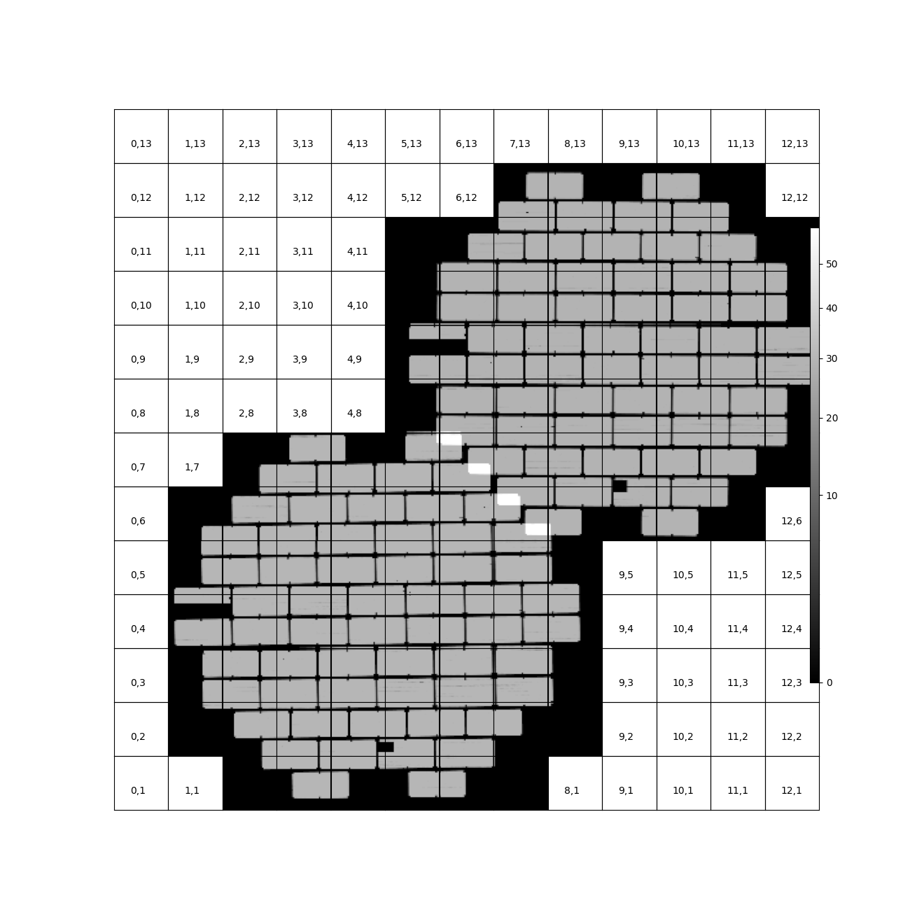
Fig. 31 Overview mosaic of the number of g-band images coadded for both fields from 2015.#
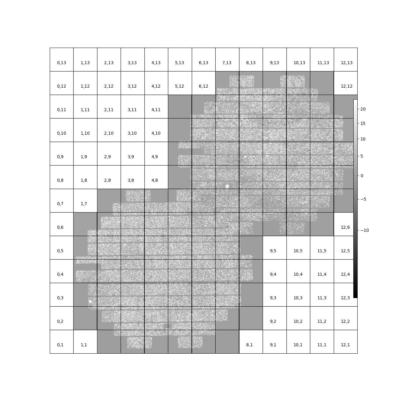
Fig. 32 Overview mosaic of the g-band coadded deep images for both fields from 2015.#

Fig. 33 Overview mosaic of the number of i-band images coadded for both fields from 2015.#
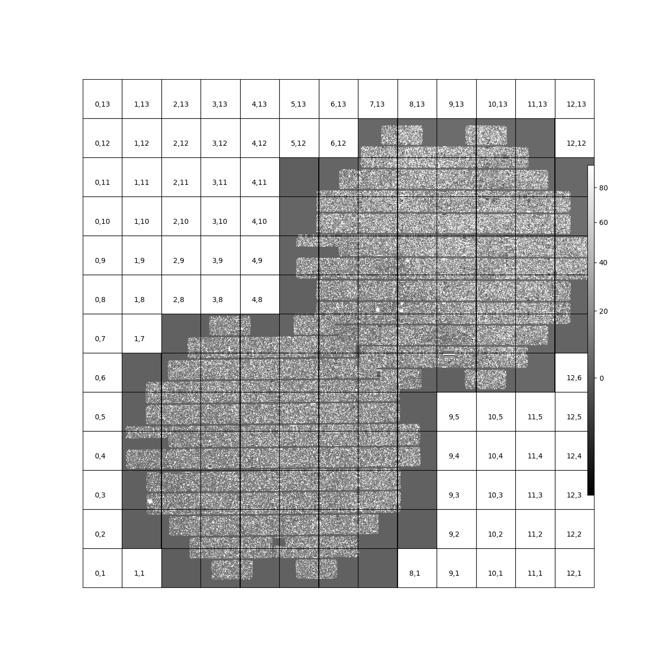
Fig. 34 Overview mosaic of the i-band coadded deep images for both fields from 2015.#
Image differencing and ap_pipe#
The initial stages of ap_pipe perform Single Frame Processing, and face the same challenges detailed above.
After processing the science image, the next step is to create a template and perform image differencing.
We have no concerns about creating the template, but if we get overlapping source residuals from image differencing it could be very challenging to detect and measure real transients and variable sources.
In Fig. 35 - Fig. 40 below we show the science image, the warped template prior to PSF matching, and the resulting image difference for a g-band and an i-band observation.
For this example, the science images are both from the 2013 observing run, using templates built from the better-seeing 2015 observations.
In both cases the science image has slightly worse seeing than the template, allowing us to use the Alard and Lupton [1998] image differencing algorithm in the standard convolution mode.
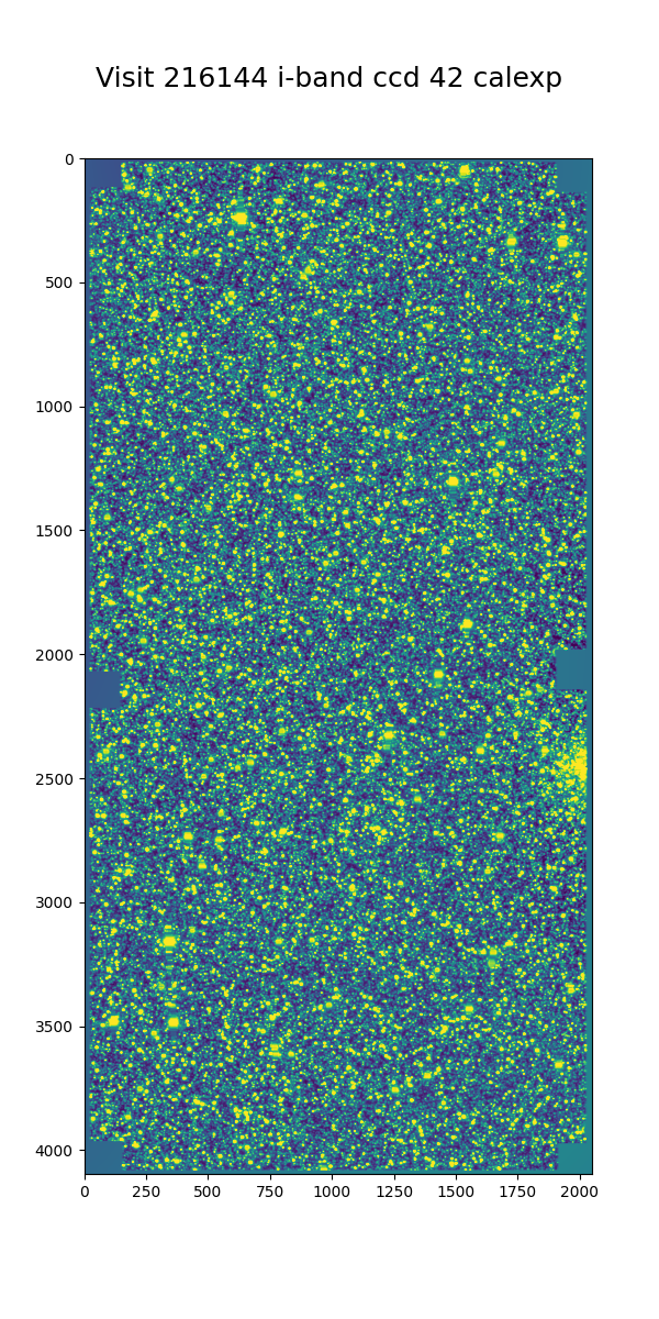
Fig. 35 I-band science visit 216144 ccd 42 from 2013 B2. The color scale is locked to the scale of the template in Fig. 36#
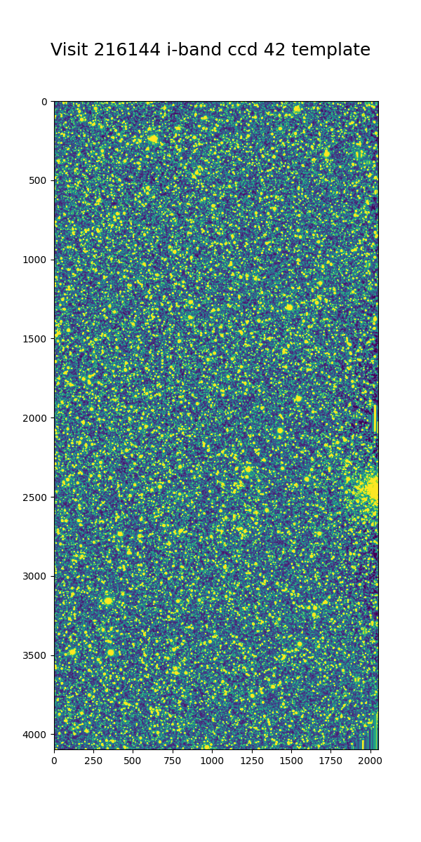
Fig. 36 Deep coadd template for i-band visit 216144 ccd 42. The color scale uses a Asinh stretch to emphasize faint features.#
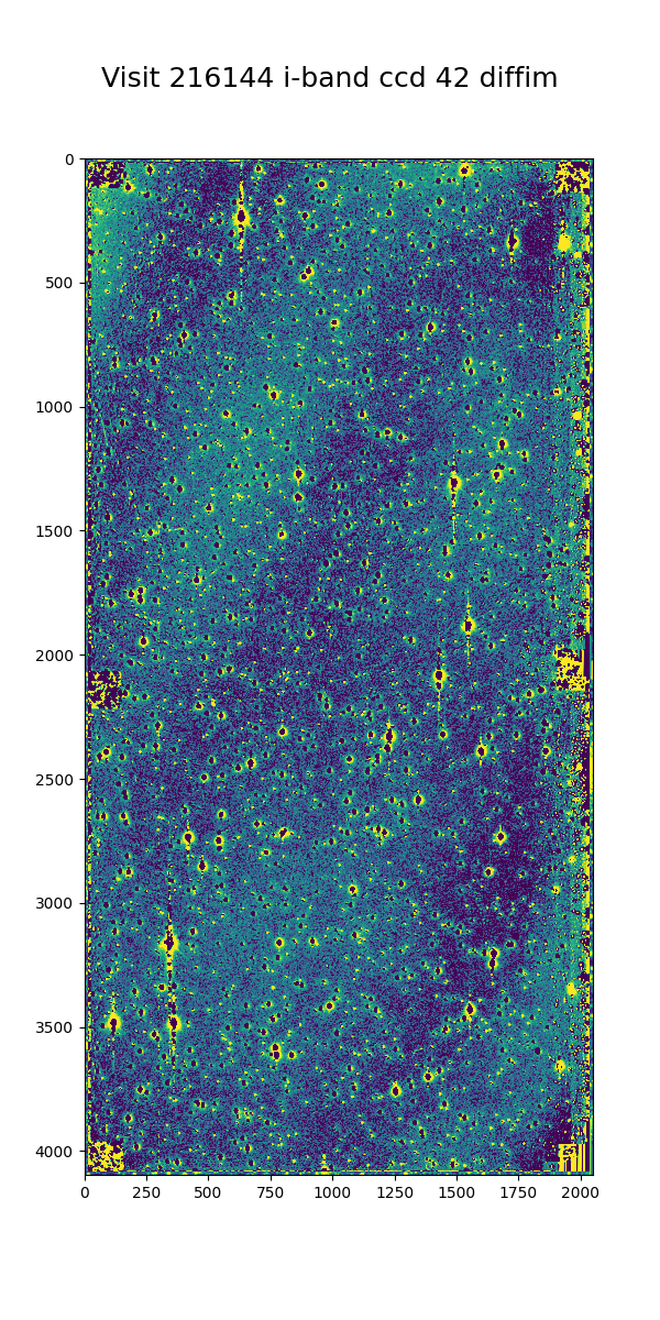
Fig. 37 Image difference for i-band visit 216144 ccd 42. The color scale is locked to the scale of the template in Fig. 36#
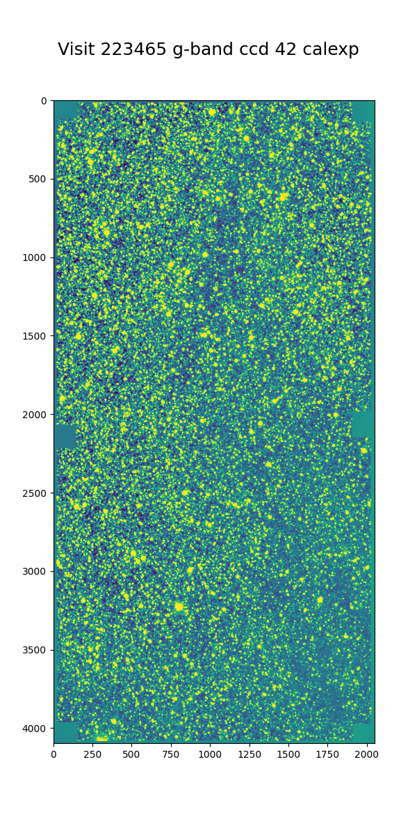
Fig. 38 G-band science visit 223465 ccd 42 from 2013 B2. The color scale is locked to the scale of the template in Fig. 39#
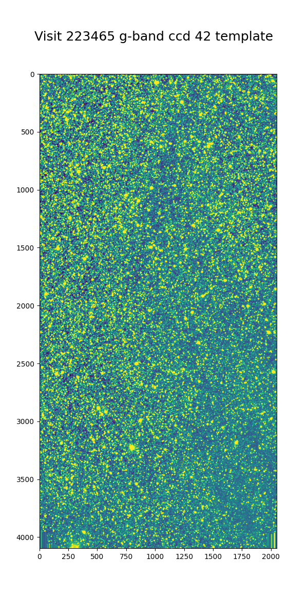
Fig. 39 Deep coadd template for g-band visit 223465 ccd 42. The color scale uses a Asinh stretch to emphasize faint features.#
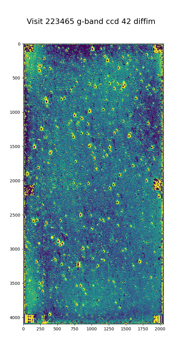
Fig. 40 Image difference for g-band visit 223465 ccd 42. The color scale is locked to the scale of the template in Fig. 39#
Several features are apparent from the above images. Most importantly, despite the sea of overlapping sources in the input images and the imperfect subtraction, the resulting DIASources are still isolated. Thus, we can still detect and measure sources in the difference image, though we have far more to deal with than for a typical observation. Most of the DIASources show artifacts characteristic of imperfect subtraction, such as dipoles and ringing patterns. The improvements that the Alert Production team is currently working on should result in better subtractions for crowded fields as well.
Conclusions and future work#
This investigation has stress-tested the LSST Science Pipelines, and uncovered several algorithmic components that need attention. Some of those improvements, such as upgrading the PSF determiner, were necessary to process the data and have already been completed. Others, such as the fidelity of image differencing, had been previously identified and the improvements are under active development.
Summary of the challenges to processing crowded fields identified in this analysis:
The PSF determiner was upgraded to PSFex, which is able to run on crowded fields. However, it does not appear to be able to model the wings of the PSF (see Fig. 5 through Fig. 12).
The cosmic ray detection and repair algorithm still fails for some ccds, and will require either careful tuning of the existing parameters or a more sophisticated implementation.
Photometric calibration is at times inconsistent, with offsets of several magnitudes in the worst cases (Fig. 17 - Fig. 24). If this is due to poor flux measurements it will likely improve with a better PSF model, but that will require further study.
We are able to measure sources at densities greater than 500,000 per square degree under good conditions, and the source counts suggest that we are not undercounting sources.
In future processing of these data we will use newly-developed pipelines to inject fake sources in the analysis to measure completeness, and we will perform a systematic visual inspection to determine purity.
The source matching algorithm will require optimization in crowded fields, as the current implementation can take over an hour to process a single ccd in extreme cases.
The quality of subtraction in image differencing remains a barrier for generating alerts. The residuals around bright sources do appear isolated, but the number of false detections is too high.
Once we have made progress on the above challenges, we could revisit the analysis of these fields. Crowded fields will present the most difficult conditions for PSF measurement and image differencing, but improvements in both components are underway.
References#
Charles F. Claver and The LSST Systems Engineering Integrated Project Team. LSST System Requirements (LSR). Systems Engineering Controlled Document LSE-29, NSF-DOE Vera C. Rubin Observatory, September 2017. URL: https://ls.st/LSE-29.
Charles F. Claver and The LSST Systems Engineering Integrated Project Team. Observatory System Specifications (OSS). Systems Engineering Controlled Document LSE-30, NSF-DOE Vera C. Rubin Observatory, January 2018. URL: https://ls.st/LSE-30.
K. Suberlak, C. Slater, and Ž. Ivezić. LSST Fall 2017 Crowded Fields Testing. Data Management Technical Note DMTN-077, NSF-DOE Vera C. Rubin Observatory, April 2018. URL: https://dmtn-077.lsst.io/.
Ian Sullivan and Eric Bellm. Fall 2020 status of crowded field processing with the LSST Alert Production Pipelines. Data Management Technical Note DMTN-171, NSF-DOE Vera C. Rubin Observatory, March 2021. URL: https://dmtn-171.lsst.io/.
C. Alard and Robert H. Lupton. A Method for Optimal Image Subtraction. ApJ, 503(1):325–331, August 1998. arXiv:astro-ph/9712287, doi:10.1086/305984.
Rubin Observatory Science Pipelines Developers. The LSST Science Pipelines Software: Optical Survey Pipeline Reduction and Analysis Environment. Project Science Technical Note PSTN-019, NSF-DOE Vera C. Rubin Observatory, September 2025. URL: https://pstn-019.lsst.io/, doi:10.71929/rubin/2570545.
Abhijit Saha, A. Katherina Vivas, Edward W. Olszewski, and others. Mapping the Interstellar Reddening and Extinction toward Baade\textquoteright s Window Using Minimum Light Colors of ab-type RR Lyrae Stars: Revelations from the De-reddened Color-Magnitude Diagrams. ApJ, 874(1):30, March 2019. arXiv:1902.05637, doi:10.3847/1538-4357/ab07ba.
E. F. Schlafly, G. M. Green, D. Lang, and others. The DECam Plane Survey: Optical Photometry of Two Billion Objects in the Southern Galactic Plane. ApJS, 234(2):39, February 2018. arXiv:1710.01309, doi:10.3847/1538-4365/aaa3e2.